There is more to Excel than you realise

In this post I share three of my favourite Excel tips that - once you know how - become very useful. Most people who use Excel have only just scratched the surface, if you take the time to learn more about Excel, you could really achieve a lot more at work and at home. Learning Excel is time consuming, and a near impossible task to do on your own. We provide regular Excel resources and tips on the blog, but nothing beats hands-on, classroom based Excel training.

Here are three Excel tips that come in handy once you know what you're doing:

How to Shade Every Other Row

When you have a long list of data that stretches across the page it can sometime be difficult to read each line precisely across. One way to help you, and your eyes, is to make every other row a different colour.

• Highlight all the rows you want to make easier to read
• Click Conditional Formatting in the 'Styles' section of the ribbon
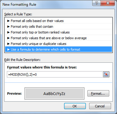
• Select New Rule > Use a formula to determine which cells to format
• In the box marked 'Format values where this formula is true enter the formula =MOD(ROW(),2)=0
• Click on the 'Format' box to apply your desired styling to every other line.
• For simple shading, click on the 'Fill' tab and click on the lightest grey.
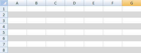
• Apply the conditional formatting and your spreadsheet should now be nice and stripy, and more importantly - easy to read:

How to Add a Drop Down List

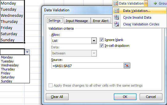
Adding a drop down list to your spreadsheets not only looks good, but it also helps stop the wrong data being entered into the system. In this example, we're going to use days on the week:

• Start off by entering all the days in a row, one day in each cell – e.g. cells A1 to A7
• Select the cell where you want the drop down list to be located
• On the Data tab click Data Validation – this will bring the Data Validation box up on the Settings tab
• In the Allow fields select List
• In the Source field you want to put where the list data is, in this case – D1 to D7
• Click okay and you will see a drop down arrow where you placed the list

How to Hide your Formulas

When you click on a cell which contains a formula then the formula appears at the top, but sometimes you may want to hide it because it’ll look neater and/ or you don’t want others copying your complex formulas.

• Click Find & Select on the Home tab and click Go To Special
• Select the Formulas option and make sure all the boxes are checked
• Click OK and Excel will highlight all cells with formulas in
• Next click Format > Format Cells > Protection and tick the Hidden box (Locked should already be ticked)
• Bring up Go To Special again and this time select Constants with all the boxes checked
• Click OK and Excel will highlight all cells without formulas in
• Bring up Format Cells > Protection again and un-check Locked and Hidden.

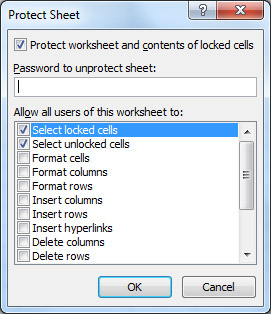
Now the formula cells are set as Hidden and the cells without formulas in are set as Unlocked, but this is all useless unless the spreadsheet is protected, to do this you will have to click Review > Protect Sheet, this should protect the sheet and if you want an added bit of security you can set a password.

Image by fdecomite on Flickr